Introduction to LSTM-based Calibration (One-Line Usage)

Author

Sima Najafzadehkhoei

Published

January 28, 2026

Overview

This vignette shows how to: 1) simulate an epidemic using epiworldR, and
2) obtain calibrated SIR parameters using calibrate_sir() from epiworldRcalibrate.

✅ No Python setup required. The package initializes the Python model internally the first time you call calibrate_sir() and cleans up automatically when asked.

Libraries

library(tidyverse)

── Attaching core tidyverse packages ──────────────────────── tidyverse 2.0.0 ──
✔ dplyr     1.1.4     ✔ readr     2.1.5
✔ forcats   1.0.0     ✔ stringr   1.5.1
✔ ggplot2   4.0.1     ✔ tibble    3.2.1
✔ lubridate 1.9.3     ✔ tidyr     1.3.1
✔ purrr     1.0.4     
── Conflicts ────────────────────────────────────────── tidyverse_conflicts() ──
✖ dplyr::filter() masks stats::filter()
✖ dplyr::lag()    masks stats::lag()
ℹ Use the conflicted package (<http://conflicted.r-lib.org/>) to force all conflicts to become errors

library(ggplot2)
library(patchwork)
library(epiworldR)

Thank you for using epiworldR! Please consider citing it in your work.
You can find the citation information by running
  citation("epiworldR")

Attaching package: 'epiworldR'

The following object is masked from 'package:lubridate':

    today

library(epiworldRcalibrate)

Ground-Truth Parameters and Simulation

We draw a single SIR parameter set and simulate 60 days.

set.seed(122)

# Draw a single parameter set
n_value <- sample(5000:10000, 1)
preval   <- runif(1, 0.007, 0.02)
crate    <- runif(1, 1, 5)
recov    <- runif(1, 0.071, 0.25)
R0_true  <- runif(1, 1.1, 5)
ptran    <- R0_true * recov / crate

true_params <- tibble(
  n = n_value,
  prevalence = preval,
  contact_rate = crate,
  transmission_rate = ptran,
  recovery_rate = recov,
  R0 = R0_true
)

true_params

# A tibble: 1 × 6
      n prevalence contact_rate transmission_rate recovery_rate    R0
  <int>      <dbl>        <dbl>             <dbl>         <dbl> <dbl>
1  6967     0.0188         1.76             0.149        0.0783  3.36

ndays <- 60
true_model <- ModelSIRCONN(
  name = "true_simulation",
  n = true_params$n,
  prevalence = true_params$prevalence,
  contact_rate = true_params$contact_rate,
  transmission_rate = true_params$transmission_rate,
  recovery_rate = true_params$recovery_rate
)
run(true_model, ndays = ndays)

_________________________________________________________________________
|Running the model...
|||||||||||||||||||||||||||||||||||||||||||||||||||||||||||||||||||||||| done.
|

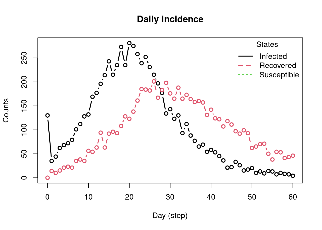
# Extract daily incidence (length must be 61: day 0..60)
inc_plot <- plot_incidence(true_model, plot = TRUE)

incidence_ts <- inc_plot[, 1]
length(incidence_ts)  # should be 61

[1] 61

Calibrate SIR Parameters (One line)

calibrate_sir() automatically:

initializes the BiLSTM model (if not already loaded),
preprocesses the series,
predicts ptran, crate, and R0,
and returns a named vector.

lstm_predictions <- calibrate_sir(
  daily_cases = incidence_ts,
  population_size = true_params$n,
  recovery_rate = true_params$recovery_rate
)

Using existing virtual environment: epiworldRcalibrate

Package 'numpy' found

Package 'sklearn' found

Package 'joblib' found

Package 'torch' found

Verifying package installation...

✓ numpy v2.2.6 loaded successfully

✓ sklearn v1.7.2 loaded successfully

✓ joblib v1.5.2 loaded successfully

✓ torch v2.9.1+cpu loaded successfully

All required Python packages are ready!

BiLSTM model loaded successfully.

cat("LSTM Parameter Predictions:\n")

LSTM Parameter Predictions:

lstm_predictions

    ptran     crate        R0 
0.1087724 2.4655740 3.4240935

Turn predictions into a tidy frame for comparison:

lstm_params <- tibble(
  n = true_params$n,
  prevalence = true_params$prevalence,
  contact_rate = lstm_predictions[["crate"]],
  transmission_rate = lstm_predictions[["ptran"]],
  recovery_rate = true_params$recovery_rate,
  R0 = lstm_predictions[["R0"]]
)

params_comparison <- bind_rows(
  true_params %>% mutate(param_type = "true"),
  lstm_params %>% mutate(param_type = "lstm")
)

params_comparison

# A tibble: 2 × 7
      n prevalence contact_rate transmission_rate recovery_rate    R0 param_type
  <int>      <dbl>        <dbl>             <dbl>         <dbl> <dbl> <chr>     
1  6967     0.0188         1.76             0.149        0.0783  3.36 true      
2  6967     0.0188         2.47             0.109        0.0783  3.42 lstm

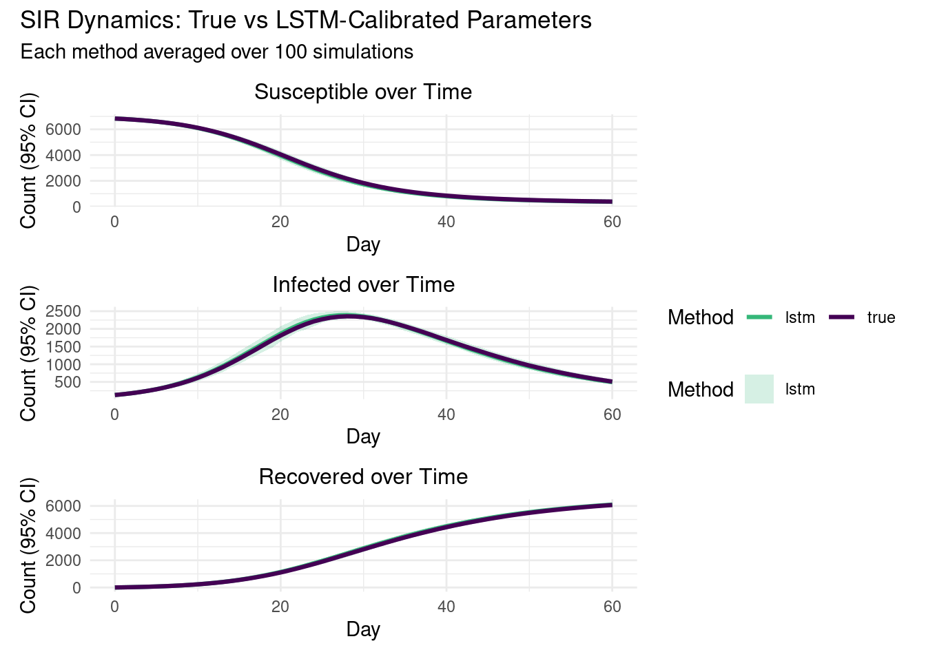
Forward Simulations: True vs LSTM Parameters

We run multiple replicates with the true parameters and with the LSTM-calibrated parameters to compare dynamics.

n_reps <- 100
all_simulation_results <- tibble()

for (i in seq_len(nrow(params_comparison))) {
  row <- params_comparison[i, ]

  forward_model <- ModelSIRCONN(
    name = paste0("forward_", row$param_type),
    n = row$n,
    prevalence = row$prevalence,
    contact_rate = row$contact_rate,
    transmission_rate = row$transmission_rate,
    recovery_rate = row$recovery_rate
  )

  saver <- make_saver("total_hist")
  run_multiple(forward_model, ndays = ndays, nsims = n_reps, saver = saver, nthreads = 8)
  results <- run_multiple_get_results(forward_model, nthreads = 2)

  sim_data <- results$total_hist %>%
    group_by(date, state) %>%
    summarize(
      mean_count = mean(counts),
      ci_lower   = quantile(counts, 0.025),
      ci_upper   = quantile(counts, 0.975),
      .groups = "drop"
    ) %>%
    mutate(param_type = row$param_type)

  all_simulation_results <- bind_rows(all_simulation_results, sim_data)
}

Starting multiple runs (100) using 8 thread(s)
_________________________________________________________________________
_________________________________________________________________________
||||||||||||||||||||||||||||||||||||||||||||||||||||||||||||||||||||||||| done.
Starting multiple runs (100) using 8 thread(s)
_________________________________________________________________________
_________________________________________________________________________
||||||||||||||||||||||||||||||||||||||||||||||||||||||||||||||||||||||||| done.

Visualize S, I, R Trajectories

method_colors <- c("true" = "#440154FF", "lstm" = "#35B779FF")

create_sir_plot <- function(data, state_name, title) {
  plot_data <- data %>% filter(state == state_name)
  ggplot(plot_data, aes(x = date, color = param_type)) +
    geom_ribbon(
      data = plot_data %>% filter(param_type == "lstm"),
      aes(ymin = ci_lower, ymax = ci_upper, fill = param_type),
      alpha = 0.2, color = NA
    ) +
    geom_line(aes(y = mean_count), linewidth = 1.1) +
    scale_color_manual(values = method_colors) +
    scale_fill_manual(values = method_colors) +
    labs(title = title, x = "Day", y = "Count (95% CI)", color = "Method", fill = "Method") +
    theme_minimal() +
    theme(legend.position = "bottom", plot.title = element_text(size = 12, hjust = 0.5))
}

p_sus <- create_sir_plot(all_simulation_results, "Susceptible", "Susceptible over Time")
p_inf <- create_sir_plot(all_simulation_results, "Infected",    "Infected over Time")
p_rec <- create_sir_plot(all_simulation_results, "Recovered",   "Recovered over Time")

(p_sus / p_inf / p_rec) + plot_layout(guides = "collect") +
  plot_annotation(
    title = "SIR Dynamics: True vs LSTM-Calibrated Parameters",
    subtitle = paste0("Each method averaged over ", n_reps, " simulations")
  )

Bias Tables

Parameter Bias

param_bias <- tibble(
  Parameter = c("Contact Rate", "Transmission Rate", "R0"),
  True = c(true_params$contact_rate, true_params$transmission_rate, true_params$R0),
  LSTM = c(lstm_params$contact_rate, lstm_params$transmission_rate, lstm_params$R0)
) %>%
  mutate(
    Bias = LSTM - True,
  )

param_bias

# A tibble: 3 × 4
  Parameter          True  LSTM    Bias
  <chr>             <dbl> <dbl>   <dbl>
1 Contact Rate      1.76  2.47   0.703 
2 Transmission Rate 0.149 0.109 -0.0405
3 R0                3.36  3.42   0.0657